Group Data into Buckets or Calculate Ratios with a single SQL Query

How do you calculate a certain ratio with a single SQL query? How do you group users into buckets with SQL? These appear to be common interview questions for Data Analyst roles and can be easily done using the CASE statement. You can think of CASE statements as something similar to if/else statements in various programming languages.

If you do not have SQL installed on your computer, you can use SQL Fiddle to test out your queries on the web. In this post, I will be using MySQL. Let’s try the queries out with some mock data.

Building an Online Recommender System

In this post, I will write about how I created a web application for the recommender system I built in the previous post using the Shiny package in R.

Building a Movie Recommendation Engine with R

I decided to work on a movie recommendation engine since it seems like one of the first pet projects machine learning classes tend to recommend (like in this Udacity course). In this post, I will attempt to use both the Content-based Filtering approach and the Collaborative Filtering approach to build a basic movie recommendation engine.

Measures of Similarity and Distance

Similarity and Distance is a numerical way to measure how alike or geometrically close two data objects are. Scenarios where you might want to calculate similarity and distance would be when you are trying to identify groups of users who have similar behavior or usage patterns. There are several ways of measuring similarity and distance, and also several R packages out there that does the job for you, such as the sets package or the proxy package.

In this post, I’m going to cover 3 measures of similarity/distance.

1) Jaccard Similarity Coefficient. Jaccard’s Coefficient is a measure of similarity, as apposed to Jaccard’s Distance, which is a measure of dissimilarity. The Jaccard’s Coefficient is good for measuring similarity of binary data. The Jaccard’s Coefficient formula is represented as follows:

where given 2 binary objects p and q:

M₀₁ = the number of attributes where p was 0 and q was 1
M₁₀ = the number of attributes where p was 1 and q was 0
M₁₁ = the number of attributes where p was 1 and q was 1
M₀₀ = the number of attributes where p was 0 and q was 0

Since we are working with binary data, the above will be every combination possible for every pair of data points in p and q. Note that M₀₀ is not a part of the formula. This is due to how Jaccard similarity is based on joint presence, and so M₀₀ was not included.

Like most measures of similarity, the Jaccard Similarity Coefficient will return a number ranging from 0 to 1, with 1 being the most similar and 0 being the least similar. Jaccard’s Distance, being a measure of dissimilarity, will require an opposite interpretation — 1 is the most dissimilar and 0, the least dissimilar.

Jaccard’s Coefficient also works for non-binary data, but it will be computed differently using the below formula:

2) Euclidean Distance. The Euclidean Distance is a commonly used distance measurement. It represents the geometric distance between the corresponding points in 2 vectors. The Euclidean Distance is calculated as follows:

where n is the number of attributes in your dataset and p_k and q_k are the k^th attributes of data objects p and q.

A large limitation of the Euclidean Distance is that it assumes that all variables in your dataset are in the same units, which isn’t the case for most datasets. For example, you could have weight and height in the same dataset, and these attributes are measured with different units and are not directly comparable. The Euclidean Distance also doesn’t take correlation of attributes into consideration.

3) Mahalanobis Distance. The Mahalanobis Distance removes several of the limitations of the Euclidean Distance. It might be a good idea to use the Mahalanobis Distance if your data shows high correlation between attributes or if your data is in different units or scales. It takes into account the variance of each variable, and the covariance between variables.

(x – μ)^T Σ ^-1 (x – μ)

Naturally, there are also downsides to using the Mahalanobis Distance over Euclidean Distance. The computation time and memory requirement for the former is significantly larger than the latter. Also, it might be difficult to compute the covariance matrices.

sources: here, here

Unsupervised Learning – K-means Clustering

Clustering is a kind of unsupervised learning where we try to identify similarities and patterns from unlabeled data. Data points which exhibit similarities are grouped together into a cluster, and there is no fixed way these data points can be separated — clustering is subjective. Ideally, good clusters will exhibit high intra-class similarity and low inter-class similarity. This would mean that the maximum distance between points within a cluster will be small, but the distance between clusters is large. There are several ways to determine similarity, which shall be covered in a separate blog post.

Random Restart Hill Climbing Algorithm

Advantages of Random Restart Hill Climbing:
Since you randomly select another starting point once a local optimum is reached, it eliminates the risk that you find a local optimum, but not the global optimum. Also, it is not much more expensive than doing a simple hill climb as you are only multiplying the cost by a constant factor — number of times you want to do a random restart.

Disadvantages of Random Restart Hill Climbing:
If your random restart point are all very close, you will keep getting the same local optimum. Care should be taken that the next random restart point should be far away from your previous. This would allow a more systemic approach to random restarting.

Running R on Amazon EC2 quickly with Amazon Machine Images

With its many useful inbuilt packages and its ease of use, R has become increasingly popular as a tool for data analysis. Users are able to perform complex statistical analyses or machine learning algorithms on their data easily. However, not all is sunshine and rainbows — R stores all objects in memory. This means that you will need lots of RAM and computational power in order to analyze larger datasets.

I quickly faced this memory limitation problem in R while playing around with some larger datasets that had about 4 million rows. In a bid to overcome the long waiting times for something to process, I began looking for extra computational resources in the cloud. That’s when i stumbled across Louis Aslett’s website. You can easily create an EC2 instance that runs RStudio using these Rstudio server Amazon Machine Images (AMIs). Of course, there are also ways to set up your own Rstudio environment on your own, but using an AMI makes the process easier for those who are not so Linux-savvy.

Steps to setting up your Rstudio environment on EC2:
1) Get an Amazon account. It can be the same account you use to shop on Amazon.com

2) Log in to the Amazon AWS Console

3) Choose one of the AMIs available on Louis Aslett’s website based on your region

4) Choose an EC2 Instance Type. Note that only the t2.micro is free tier eligible. It’s best to get acquainted with the fees and resources available for each instance type before beginning. You only get 1 year of free use for the t2.micro and it only offers 1 GiB of memory. After you’re done choosing, proceed to Configure Security Group.

5) Make sure you have 2 types. SSH port range 22, and HTTP port range 80. These two are the necessary to access Rstudio. When you’re done, click Launch.

5) You might get a pop-up window at this stage requesting you to select a key pair. It is important to create a key pair if you don’t already have one. Just insert a name for it and download it. This will create the pem file you’ll need to ssh into the server to access your files on the EC2 instance. After launching, click View Instances to see the instance you just initiated.

6) Select the instance that is running, and copy the Public DNS. If you paste this into your browser address bar, you should see the RStudio login page. The default username and password is both “rstudio”. Follow the instructions in the Welcome.R script to change your password, and then close the file without saving. Your Rstudio environment is now up!

Now that you have your RStudio set up on Amazon EC2, you will need to know how to move your files from your local environment into the cloud, and vice versa. This is where the key pair file your downloaded in step 5 comes into play.

How to copy files from your computer into your EC2 instance:
1) Fire up your terminal. I use iTerm on a Mac. Go to the directory where you saved the key pair file. you can do this by typing something like

cd ~/Downloads

2) Use the chmod command to change the permissions on the key pair file

chmod 400 nameofyourkeypair.pem

3) Copy your local files into your EC2 instance. You will need to include the entire file path of your key pair file, and the public DNS of your instance would be what you pasted in your browser address bar to access RStudio. Here, we are assuming you are in the same directory as where FileName.txt is saved.

scp -i ~/Downloads/nameofyourkeypair.pem FileName.txt ubuntu@your-public-DNS:~

If you receive a prompt asking if you are sure you want to continue, just type ‘yes’ and continue. Your file should be copied over

How to copy files from your EC2 instance to your computer:
1) Step 1 and 2 of the above apply as well. If you have already done this before, you can skip.

2) Enter the below command to copy files from your EC2 instance to your computer. The first file path is the location of your file in the EC2 instance, and the second file path would be where you want your file to be saved in your local environment.

scp -i ~/Downloads/nameofyourkeypair.pem ubuntu@your-public-DNS:~/FileName.txt ~/Documents/FileName2.txt

Have Fun!

Machine Learning Error Metrics – Algorithm Precision & Recall

There are many ways to measure the accuracy or error rates of your machine learning algorithm. Some frequently used error metrics are root mean square error (RMSE), root mean square log error (RMSLE), average euclidean distance, etc.

Precision and Recall are just another way of measuring error for classification problems, and they can be useful if you’re handling an imbalanced or skewed dataset. For example, if 95% of your dataset falls under Class 0, and the remaining 5% falls under Class 1 (the rare, minority class), having an error rate of 0.05 might look good, but it doesn’t mean much because you’d get the same value if you predicted every observation as Class 0. This is where Precision and Recall comes into play.

In R, you can easily come up with a frequency table that can help you calculate Precision and Recall.

table(prediction[[1]], df$classification_target)

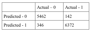
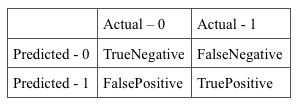
This will return you a frequency table. For easier explanation, I’ve put the results into a table. The table on the bottom right explains the figures in each quadrant.

True Negatives: observations which are Class 0, and were correctly classified as 0
True Positives: observations which are Class 1, and were correctly classified as 1
False Positives: observations which are Class 0, but were wrongly classified as 1
False Negatives: observations which are Class 1, but were wrongly classified as 0

Precision: Of all observations which we predicted Class 1 for, which of them are actually Class 1?

Recall: Of all observations that are actually Class 1, what fraction of them are correctly predicted as Class 1?

Precision and Recall will give a more accurate evaluation of how well your classifier is doing, especially in the case of skewed/imbalanced datasets. Classifiers with high precision and high recall can be viewed as a good classifier.

Reverse Geocoding

This is the Python code written to perform Reverse Geocoding — a process to convert latitudes and longitudes into a human-readable address. This was done with the help of the pygeocoder Python library, a Python wrapper for the Google Geocoding API. As I was working with a dataset that had a column containing latitudes and longitudes, I thought it made sense to perform Reverse Geocoding so I could easily identify which rows were applicable to the US state that I was interested in with a simple grep. Unfortunately, the method failed me as the Google Geocoding API has a limit of 2,500 free queries every 24 hours, and I was looking at a dataset that was almost 200,000 rows long. Any further queries were promptly banned by Google. This would only be useful for small datasets.

from pygeocoder import Geocoder
import os
import time
import codecs
import unicodedata

with open('quakedataA') as f:
    content = f.readlines()

for lines in content:
    col = lines.split(',')
    lat = float(col[1])
    llong = float(col[2])

    success = True
    try:
        results = Geocoder.reverse_geocode(lat, llong)
        time.sleep(0.1)
    except Exception as e:
        print e

    my_file = codecs.open('quake_data_geocodedA.txt', 'a', encoding='utf8')    
    if success:
        col.append(results.formatted_address.replace('\r', '').replace('\n', ''))
        print 'col is', col
        out_string = ''
        for c in col:
            out_string += c.rstrip(os.linesep) + ','

        out_string += '\r'
        out_string.encode('ascii','xmlcharrefreplace')
        my_file.write(out_string)

Finding Coordinates within California’s Boundaries — Ray Casting Method

###
Here is the Python code I used to identify the points that are within California’s geographical boundaries. The coordinates used for the 4 outermost corners of the polygon are estimated locations that are situated slightly beyond the actual geographical boundaries so that we are able to capture all points in a 4-sided polygon.

The output file will contain only the data for points that fall within the identified polygon.

# Helper code found on http://geospatialpython.com/2011/01/point-in-polygon.html
# Determine if a point is inside a given polygon or not
# Polygon is a list of (x,y) pairs. This function returns True or False.
# The algorithm is called the "Ray Casting Method".

import os
def point_in_poly(x,y,poly):

n = len(poly)
inside = False

p1x,p1y = poly[0]
for i in range(n+1):
p2x,p2y = poly[i % n]
if y > min(p1y,p2y):
if y <= max(p1y,p2y):
if x <= max(p1x,p2x):
if p1y != p2y:
xints = (y-p1y)*(p2x-p1x)/(p2y-p1y)+p1x
if p1x == p2x or x <= xints:
inside = not inside
p1x,p1y = p2x,p2y

return inside

polygon = [(41.979656,-125.678101),(41.995733,-119.761963),(32.888237,-112.763672),(31.521191,-119.443359)]

with open('quake_data.txt') as f:
content = f.readlines()

for lines in content:
col = lines.split(',')
lat = float(col[1])
llong = float(col[2])

## Call the function with the points and the polygon. Write results out to text file
print point_in_poly(lat,llong,polygon)
if point_in_poly(lat,llong,polygon) == False:
pass
if point_in_poly(lat,llong,polygon) == True:
out_string = ''
for c in col:
out_string += c.rstrip(os.linesep) + ','
out_string += '\r'
my_file = open('point_in_poly.txt', 'a')
my_file.write(out_string)